What exactly is AI and how does it work?

Definitions and usage examples

What is “AI”? The term “AI” has been misused and abused by the media and general public alike. Let us first set the record straight. In the strictest sense, artificial intelligence means some tasks performed by human-made machines that are based on some logic. Here are some broad examples or categories in the context of computer programmes:

If-else statements:
A set of logical instructions to a computer, designed by humans, to carry out tasks based on some conditions. For example, a simple computer programme may be: if the music volume is louder than 70 dB, decrease volume; if the music volume is quieter than 20 dB, increase volume; otherwise, do not adjust volume.
Machine learning:
This is what most people call AI these days, even though it is a sub-category of AI. Very broadly speaking, this means computer programmes designed to learn some pattern in some data. For example, let’s say we have a large dataset containing people’s country of origin, age, height, and weight. We write a computer model (numerical equations, decision tress, or something else) to analyse the data, so that when we enter someone’s country and age, we can get a prediction of the person’s height and weight. This is machine learning; we programme a computer to learn patterns in some data.

Broad categories of machine learning

Now, machine learning has many forms and complexities. Something that used to be not called machine learning at all is curve fitting. Linear regression belongs to this category. For example, given a set of measurement data (height, weight) of everybody, what is the line that fits best?

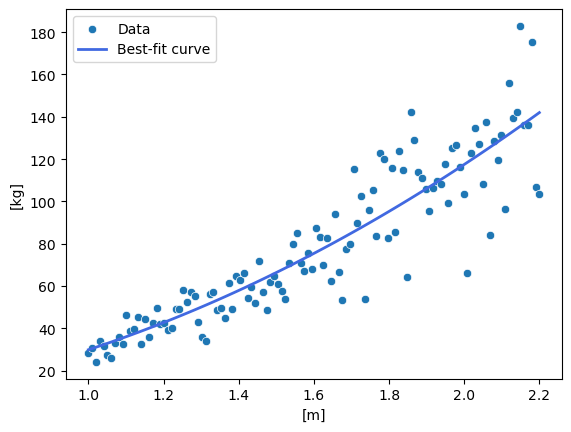
Figure 1: Some randomly-generated data and the best-fit curve

With this line (actually an equation), if we have a person’s height, we can estimate the person’s weight with some level of confidence.

Most of the time, though, the term “machine learning” refers to the following groupings:

“Classic” machine learning

I will give examples instead of being exhaustive. A commonly used type of “classic” machine learning is the decision tree, which gives rise to random forests.

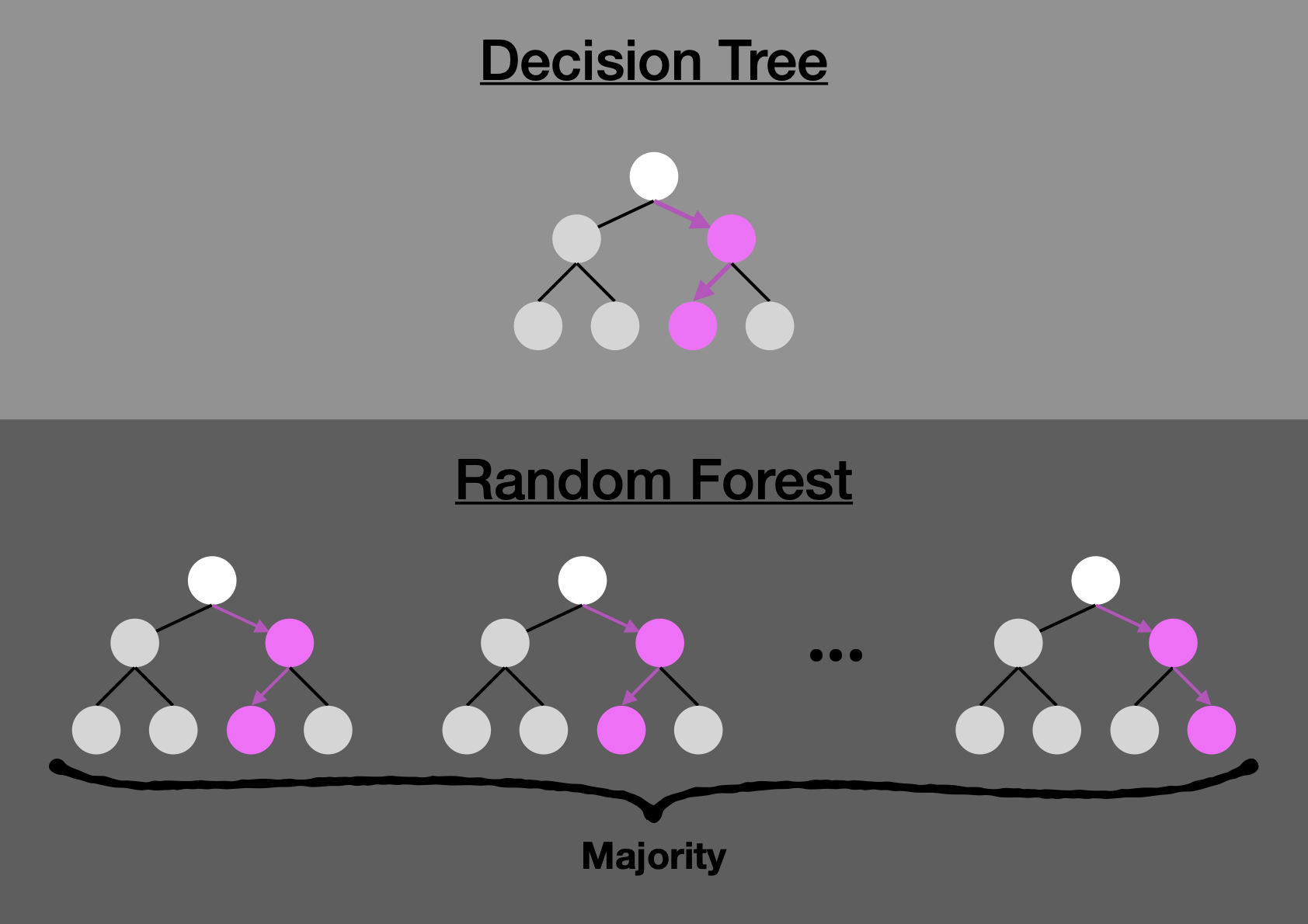
Figure 2: Top: A decision tree; bottom: A random forest consisting of many decision trees, with the final result decided by the majority.

One example usage of this type of machine learning is: Is this email a spam? One can programme a computer to take in a large database of emails labelled as genuine or spam (perhaps by users who label them, or workers tasked with such a tedious job). The computer programme can instruct the computer to use a large number of decision-tree structures (i.e., the random-forest model) for its analysis. The branches of the trees in the forest may learn to ask “is this sender known?”, “does the text contain ‘enlarge’?”, “how long is the email?”, “which IP address range?”, etc.

Deep learning: a subset of machine learning

Even though they are already very powerful, machine-learning models such as decision trees have straightforward processes. To put it very simplistically, the model learns by trying to split the data along the most distinguishing boundaries (i.e., the “decisions”) until the desired predictive categories or accuracies are reached.

There is, however, a type of machine-learning models that are much more complicated and involved many more “learnable” parameters stacked in very complex structures. These models belong to a sub-category called “deep learning”.

The most common example is the artificial neural network (ANN). Most of the popular AI tools used for facial recognition, self-driving cars, or the “scary ones” such as those generating “deep-fakes” and chatbots such as ChatGPT are all based on some form of ANN.

Complexity aside, deep-learning models, just like the “classic” machine-learning models, or even the simple curve-fitting methods, are all models in the same sense: each model is a mathematical computational construct that is fitted to some data, so that this construct (i.e., the model) can be used to make predictions that are reasonably accurate in the domain and range close enough to the original training data. (The part about domain and range is important. To give an extreme example, it is not a good idea to use the model trained on human height and weight to predict the mass and brightness of stars.)

How does it any of this work?

Despite the complexity of the most complicated deep-learning models, the foundational concept is similar to that of curve fitting. I will try to elaborate on this here, using a simple curve-fitting exercise as the basis.

In two-dimensional curve fitting, you have a set of \(M\) data points \((x_i, y_i)\) (\(i\) being the label from point \(1\) to point \(M\)), and you want the model to “learn” to take \(x\) and give you \(y\). The hope is that, once learnt, the model can give you a good prediction of \(y\) when you give it a new, unseen \(x\) in the future.

Let’s start simple. Let’s suppose my training data has three points. Let’s also suppose that I decided to make life easy by giving my model only one degree of freedom. In this case, the degree of freedom is the slope of a line that goes through the origin \((x = 0, y = 0)\). That is the only value that can change in our search for a best-fit line through the three training data points.

To begin the learning process, we need a starting guess. Typically, this is a value close to zero. Let’s choose 0.01.

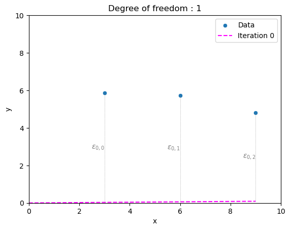
Figure 3: The three training data points, and the line of our initial guess, with a slope of 0.01 (i.e., almost a flat line).

It fits terribly. Let’s make another guess. Perhaps 0.1?

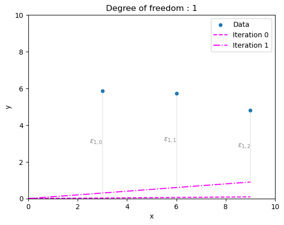
Figure 4: The three training data points, and the two guesses so far.

Slightly better. Now that we have two guesses, we can be a bit cleverer. If we calculate the absolute combined distance between the points and our first line (\(\epsilon_{0}=|\epsilon_{0,0}|+|\epsilon_{0,1}|+|\epsilon_{0,2}|\)), and do the same to our second line (\(\epsilon_{1}=|\epsilon_{1,0}|+|\epsilon_{1,1}|+|\epsilon_{1,2}|\)), we will see that \(\epsilon_{1} < \epsilon_{0}\), or that the “error” or “cost” (often also called “loss”) is getting smaller. This tells us that our next guess should have an even higher slope. If we eventually overshoot, we would see the cost increase. At that stage, we would make the next guess in the opposite direction. Eventually, with smaller and smaller adjustments, we would arrive at a best-fit line.

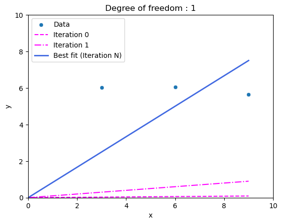
Figure 5: The three training data points, the two initial guesses, and the best-fit line (1 degree of freedom).

But it is still not very good, is it? We can do better by allowing the line to not always be crossing the origin \((0, 0)\). This kind of line has the equation of the form \(y = a\times x + b\). Now, we have two degrees of freedom, \(a\) and \(b\). The process proceeds similarly, we make an initial guess \(a_{0}\) and \(b_{0}\) and a second guess \(a_{1}\) and \(b_{1}\). Then, we check if the cost increased or decreased, and make the next guess for \(a\) and \(b\) accordingly. Eventually, after \(N\) guesses, we will arrive at a best-fit line.

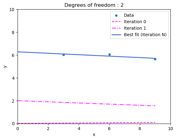
Figure 6: The three training data points, two initial guesses and the best-fit line (2 degrees of freedom).

Aside: For those who know more maths, I know there are much better ways to do this (in one step even), but I am trying to build towards how neural networks are trained.

Now, imagine our problem is not just two-dimensional. Furthermore, imagine that our problem is influenced by not just one or two parameters. We might be in a three-dimensional space with physical forces that interact (adding, multiplying, or interfering with each other), giving rise to non-linearity. In this case, the number of parameters required may go up very quickly (as an example, see this simplified model that describes viscoelastic deformation of solids).

In a lot of real-world problems, we are dealing with a much higher number of dimensions, and an even higher number of parameters tied to each dimension. Here, dimensions are mathematical instead of purely temporal-spatial, meaning that each independent aspect of the system we are trying to simulate is treated as its own mathematical dimension. In the same manner as how we went from one to two degrees of freedom above (even though we stayed with two spatial dimensions), these real-world problems require models with thousands upon thousands of parameters. In fact, a very old image-recognition model, AlexNet, from 2012 contains over 62 million parameters. How do we string together so many parameters with \(+\), \(-\), \(\times\), \(\div\)? Let’s talk about artificial neural networks now.

Neural Networks

Just like how biological neurones send signals to each other through synapses, artificial neural networks link individual parameters through mathematical operations. Using this framework of thinking, the equation above (\(a \times x + b\)) can be thought of as two neurones that takes \(x\) as an the input, link through a multiplication \(\times\) to neurone \(a\), then via an addition \(+\) to neurone \(b\), and finally producing the output value \(y\). In this case, there are two neurones that can be trained (i.e., adjusted).

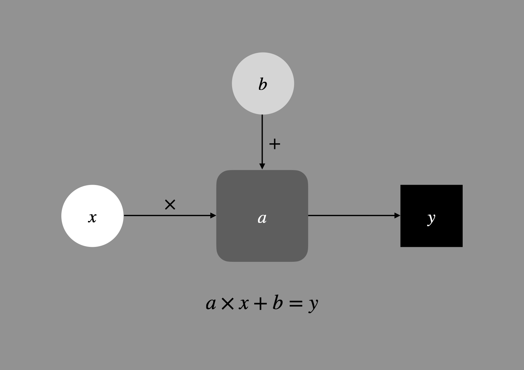Figure 7: A two-parameter neural network.

Neural networks with millions, billions, or even trillions of parameters can be built with this principle. (ChatGPT 4 is believed to have about 1.8 trillion parameters.) Complex mathematical operations such as convolution and non-linear operations could be broken down into, or built up by these simple operations (see activation functions for how non-linearity is built into neural networks through a simple “if x then y” conversion).

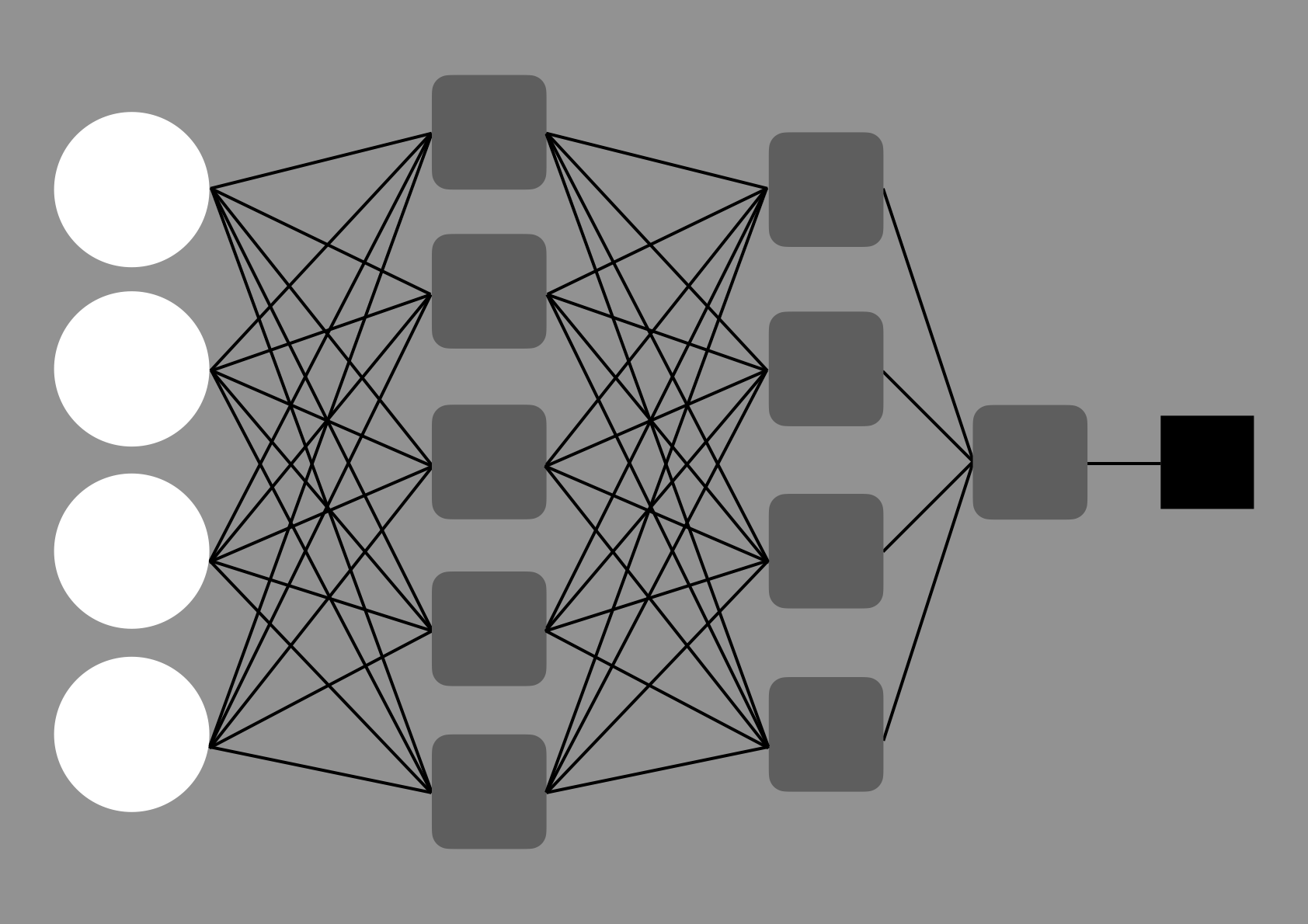
Figure 8: A few layers of neurones with a few parameters.

Even though it does take many very smart programmers to write computer programmes that can perform calculations with such a large number of mathematical operations and find the best-fit values through millions upon millions of complicated data, the underlying principle and concept is still the same as the very simplistic case we examined above. There is nothing mystical about deep-learning models such as ChatGPT or Midjourney. Complicated, yes. Mystical, no.

P.S. A brief note about explainability

The concerns about AI by experts are not about not understanding why it works, but about being able to pin-point what leads to specific outputs. In a simple regression model, such as fitting an equation \(y = a \times x + b\), it is easy to find out how some \(x\) produces some \(y\) by directly examining the equation. Models like decision trees or random forests can usually still be examined in a clear manner. For example, to find out how a random forest arrives at its output prediction, one could examine the how often a variable (or “feature”) is used in the decision trees, and how early on.

In a neural network with millions to trillions of parameters, however, this gets a bit difficult. Nevertheless, there are still methods, such as blocking out parts of the neural network and examine the impact on the outcome, or taking a sample output of an intermediate neural layer to check for particular tendencies. How to increase the clarity and explainability of AI is an area of active research (e.g. see this article for a overview of the latest research articles as of June, 2023; or search for “explainable AI” on Google Scholar).